6 Multiple Regression
6.1 Introduction
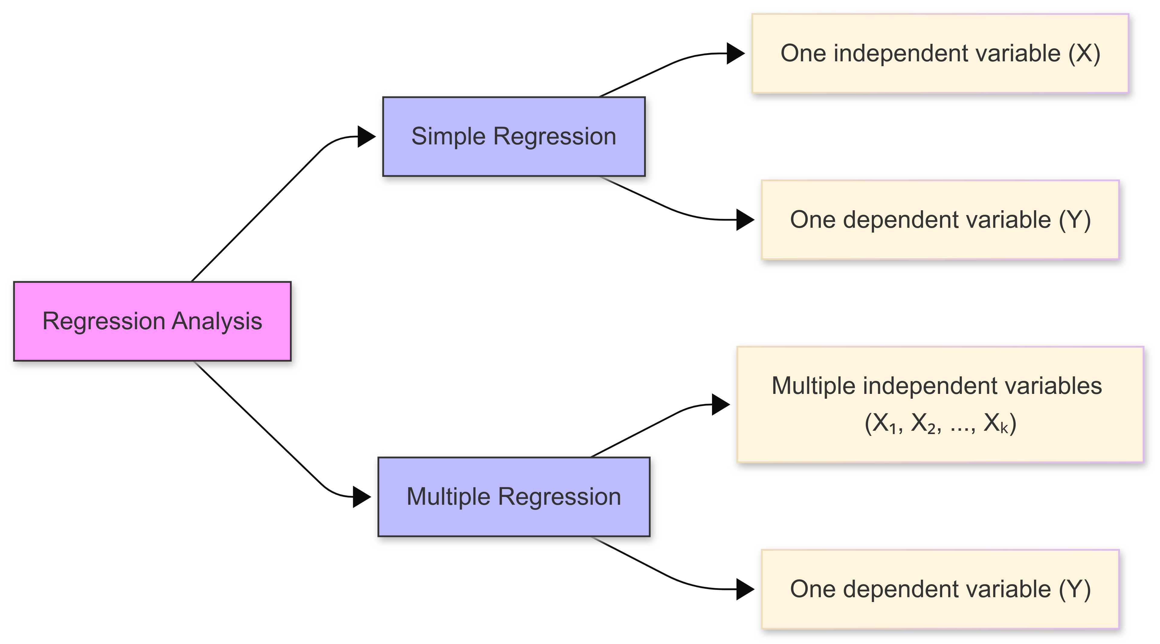
In this chapter, we deal with the topic of multiple regression. Multiple regression extends simple linear regression by analysing the relationship between a dependent variable and multiple independent variables simultaneously.
This allows us to model complex real-world phenomena where outcomes are influenced by multiple factors.
For example, in competitive swimming, an athlete’s race time (outcome) is influenced by multiple factors (stroke technique, physical conditioning, pool temperature, mental state) on race day. Understanding how these various factors work together could help coaches and athletes optimise training and performance.
Unlike simple linear regression, which considers only one predictor variable, multiple regression can incorporate numerous predictors, making it highly useful for:
- Prediction (estimating future values based on multiple input variables);
- Explanation (understanding the relative importance of different predictors); and
- Control (accounting for confounding variables in experimental research).
Formula
It’s important to understand the general form of a multiple regression model, which can be expressed as:
\[ Y = β₀ + β₁X₁ + β₂X₂ + ... + βₖXₖ + ε \]
Where:
- \(Y\) is the dependent variable
- \(β₀\) (‘beta zero’) is the intercept (constant term)
- \(β₁, β₂, ..., β\)ₖ are the regression coefficients
- \(X₁, X₂, ..., Xₖ\) are the independent variables
- \(ε\) (‘epsilon’) represents the error term
In simpler terms, this equation means that:
- The outcome we’re trying to predict (\(Y\)) equals…
- A starting point (\(β₀\)) plus…
- The effect of each predictor variable (\(β₁, β₂,\) etc.) multiplied by its value (\(X₁, X₂,\) etc.) plus…
- Some random error (\(ε\)) that we can’t predict or control
For example, if we’re predicting a student’s test score:
- \(Y\) might be the final exam score
- \(X₁\) might be hours spent studying
- \(X₂\) might be previous test average
- \(X₃\) might be hours of sleep before exam
Each \(β\) coefficient tells us how much that factor affects the final score, while \(ε\) accounts for all other unmeasured influences.
6.2 Regression Models
6.2.1 Introduction
Multiple regression extends simple linear regression by analysing the relationship between a dependent variable and multiple independent variables simultaneously.
Multiple regression makes several key assumptions that must be satisfied for our models to be considered valid and reliable:
- Linearity - the relationship between independent and dependent variables should be approximately linear;
- Independence - our observations should be independent of each other;
- Homoscedasticity - the variance of residuals should be constant across all levels of predictors;
- Normality - the residuals should follow a normal distribution; and
- No perfect multicollinearity - the independent variables in our dataset should not be perfectly correlated.
6.2.2 Modelling interactions
One of the powerful aspects of multiple regression is its ability to model interaction effects. These occur when the relationship between an independent variable and the dependent variable changes based on the level of another independent variable.
For example:
• The effect of exercise on weight loss might depend on diet quality;
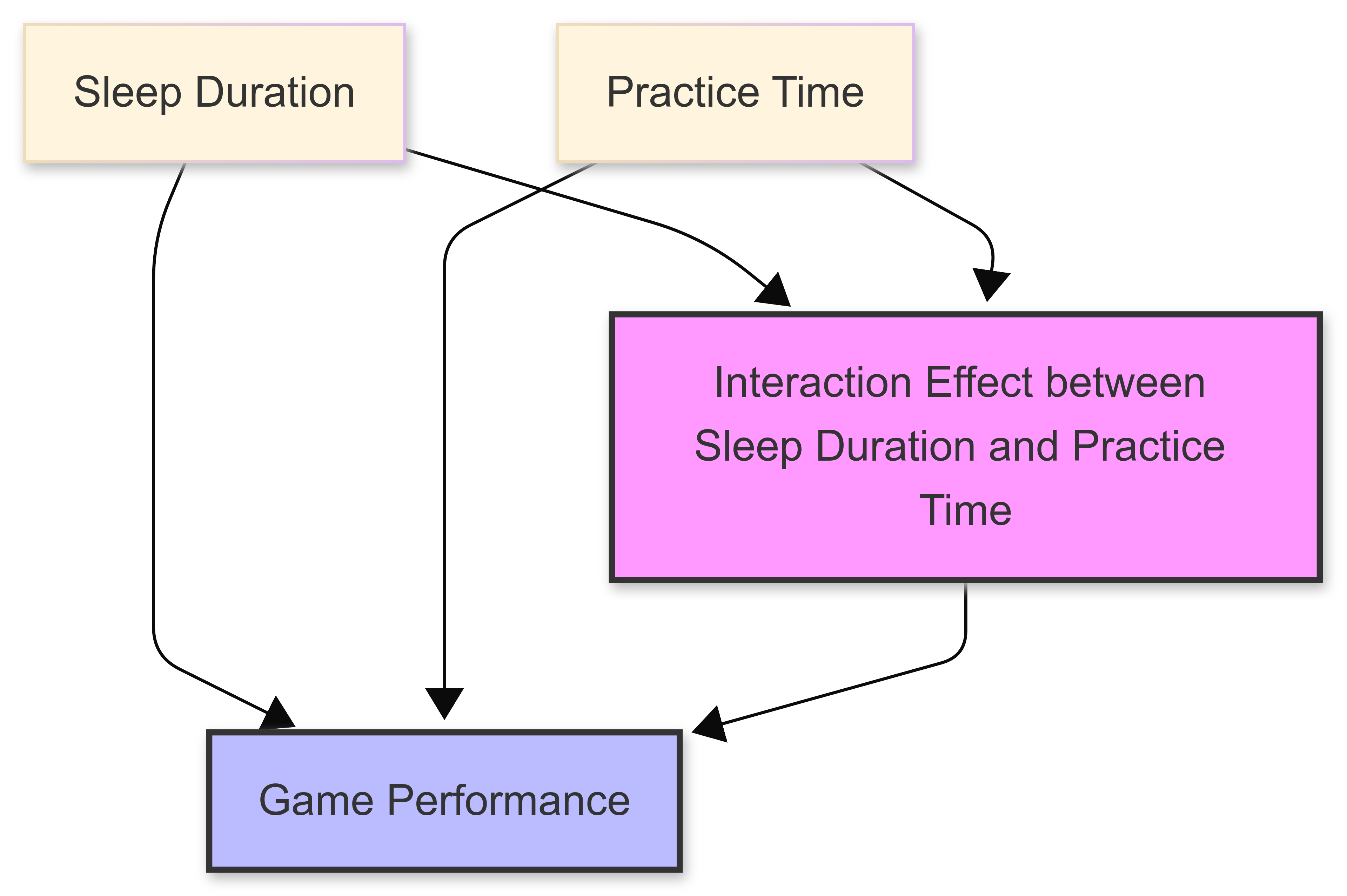
• The impact of practice time on in-game performance might vary with sleep duration; or
• The relationship between advertising spending and season ticket sales might change based on economic conditions.
6.2.3 Assumption of linearity
Recall from B1700 that ‘linearity’ describes a relationship where changes in one variable result in proportional changes in another variable. In a linear relationship, when plotted on a graph, the data points tend to follow a straight line.
The assumption of linearity is crucial in regression modelling. It suggests that the relationship between variables can be represented by a straight line equation of the form \(y = mx + b\), where:
\(m\) represents the slope (rate of change)
\(b\) represents the y-intercept (starting point)
This assumption simplifies complex relationships and makes predictions more straightforward, though it’s important to note that most real-world relationships are not truly linear!
.png)
6.2.4 Multicollinearity
Introduction
Multicollinearity occurs when two or more independent variables in a regression model are highly correlated with each other.
This can create problems in understanding the true relationship between predictors and the dependent variable.
When multicollinearity exists, it typically manifests through high correlation between predictor variables, inflated standard errors of regression coefficients, unstable coefficient estimates, and difficulty in determining individual variable importance.
Common causes
Multicollinearity can arise from several sources. Often, it’s caused by our collecting redundant variables that measure similar concepts or underlying phenomena. It can also emerge when creating polynomial terms or interaction effects in regression models.
Detection methods
Various methods are available to help us identify multicollinearity in our data:
The Variance Inflation Factor (VIF) analysis is one of the most common, and provides a numerical measure of correlation between predictors.
Other techniques include examining the correlation matrix, calculating condition numbers, and assessing tolerance values.
Solutions
Several approaches exist to address multicollinearity in statistical models:
We might choose to remove one of the correlated predictors, though this requires careful consideration of which variable to eliminate.
Another approach involves combining correlated variables into a single index.
More sophisticated solutions include using regularisation techniques like Ridge or Lasso regression, collecting additional data, redesigning the study, or employing principal component analysis (PCA) to transform the correlated variables into uncorrelated components.
Impact on analysis
While multicollinearity doesn’t affect the overall model fit or predictions, its presence can significantly impact statistical analysis. It makes it particularly challenging when we try to interpret individual coefficients accurately, as our model cannot distinguish between the effects of correlated predictors.
The issue also reduces the statistical power of the analysis and can lead to unreliable conclusions about variable importance. Multicollinearity can also cause serious problems in stepwise regression procedures, potentially leading to the selection of suboptimal models [1].
[1] D. E. Farrar and R. R. Glauber, “Multicollinearity in Regression Analysis: The Problem Revisited,” The Review of Economics and Statistics, vol. 49, no. 1, pp. 92-107, Feb. 1967.
6.2.5 Interaction effects
Introduction
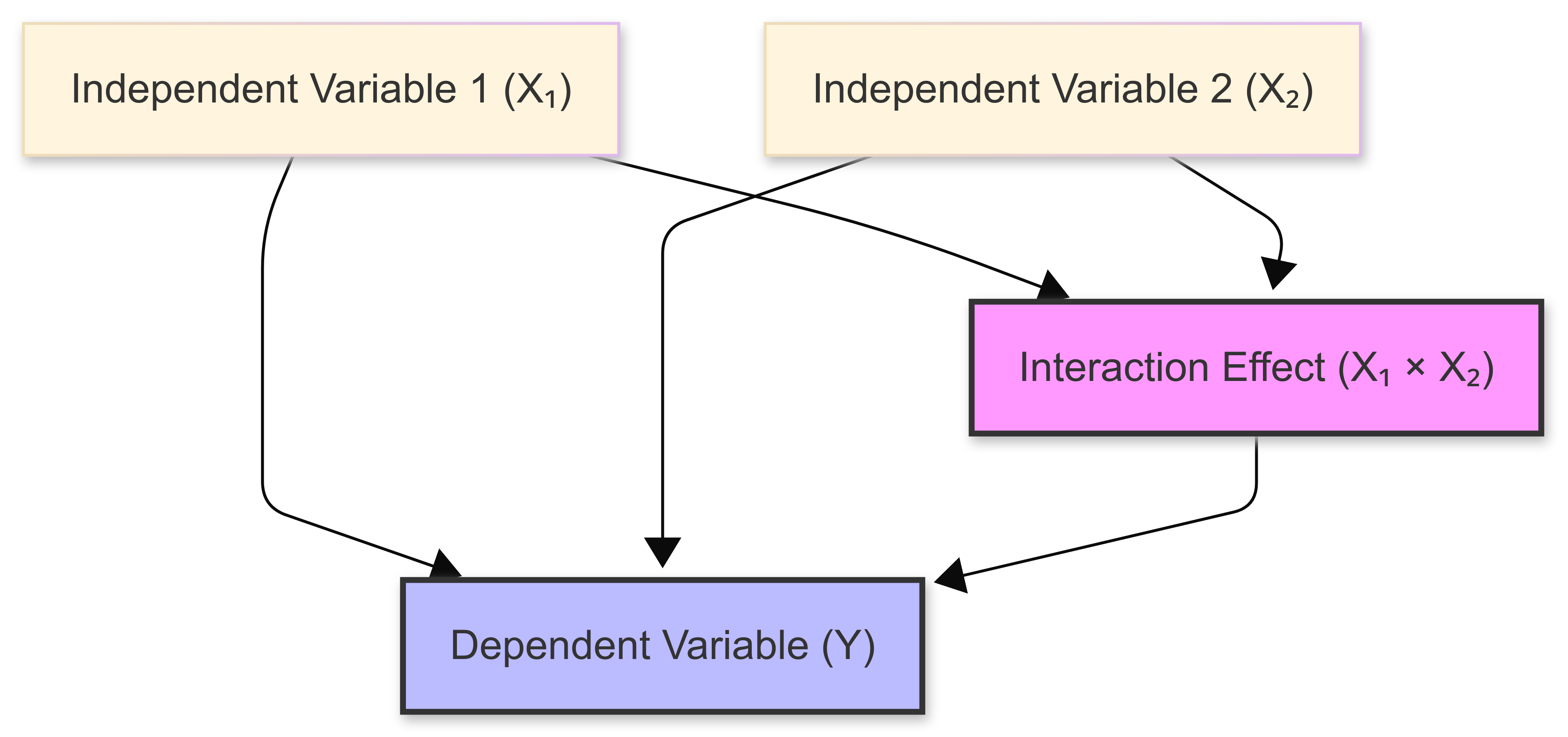
Interaction effects in multiple regression occur when the relationship between an independent variable and the dependent variable changes based on the value of another independent variable.
In the following figure, notive how the effect of one predictor variable (\(X_1\)) depends on the level of another predictor variable (\(X_2\)).
These interactions add complexity to regression models, but they can also reveal important nuances in relationships between variables that might be missed when considering only main effects.
Understanding interaction effects in our regression models is crucial for:
- Accurately modelling real-world phenomena where variables influence each other;
- Making more precise predictions by accounting for combined effects; and
- Identifying conditional relationships between variables.
Example
Consider the relationship between training intensity and athletic performance, which might be moderated by rest periods.
While both intense training and adequate rest independently contribute to performance improvement, their interaction reveals that high-intensity training is most beneficial when paired with sufficient recovery time. Conversely, intense training combined with insufficient rest could lead to decreased performance or even injury.
This interaction demonstrates why elite athletes and coaches carefully balance training intensity with recovery periods, adjusting one factor based on the level of the other to optimize performance outcomes.
Notation
Mathematically, interaction effects are represented by including product terms in the regression equation. For two variables \(X₁\) and \(X₂\), their interaction term would be \(X₁ × X₂\), indicating their joint effect on the dependent variable \(Y\).
6.3 Estimation Techniques
In multiple regression, estimation techniques are used to analyse relationships between multiple independent variables and a dependent variable.
These techniques help us determine the best-fitting model for our data, while accounting for various assumptions and data characteristics.
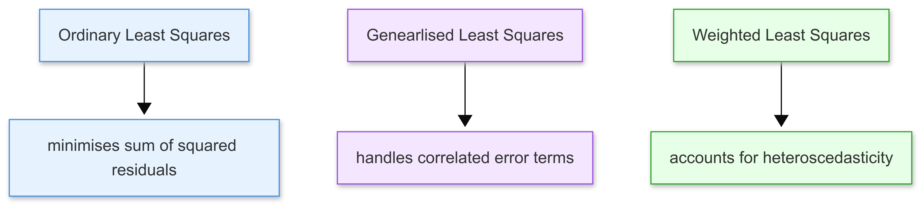
The three main estimation approaches covered in this section are:
Each technique has its own strengths and is suited to different types of data and statistical conditions.
6.3.1 Ordinary Least Squares (OLS)
Introduction
Ordinary Least Squares (OLS) is the most common estimation method used in multiple regression analysis.
The goal of OLS is to find the line of best fit that minimises the sum of the squared differences between observed values and the values predicted by the model.
This method assumes that there’s a linear relationship between the dependent and independent variables, and that the variance of the error terms is constant across all observations (homoscedasticity).
It does this by minimising the sum of the squares of the differences (residuals) between observed values and those predicted by the linear model. The ‘residuals’ are the distances from the actual data points to the line of best fit.
The following plot demonstrates this idea in the context of a simple linear regression. The regression line (the line of best fit, in red) represents how the total distance between each value (in blue) has been reduced as far as possible, by producing as small residuals as possible.
.png)
Example
Consider a dataset containing the annual income of individuals (dependent variable) and their years of education and age (independent variables). The OLS model for predicting income might be specified as follows:
\[ Income = \beta_0 + \beta_1 \times \text{Education} + \beta_2 \times \text{Age} + \epsilon \]
where \(β_0\) is the intercept, \(β_1\) and \(β_2\) are coefficients for education and age, respectively, and \(ϵ\) is the error term.
By applying OLS, we estimate the coefficients \(β0, β1, β2\) that minimise the squared differences between observed incomes and those predicted by the model.
.png)
ELI5
Imagine you’re playing a game where you need to draw a straight line through a bunch of dots on a piece of paper. You want this line to be as close as possible to ALL the dots, not just one or two of them.
That’s what OLS does…it’s like a calculator that finds the “best” line by:
Measuring how far each dot is from your line
Squaring these distances (multiplying them by themselves)
Adding all these squared distances together
Moving the line around until it finds the position where this total is as small as possible
Think of it like this: if you had a piece of string and tried to place it so it’s as close as possible to all the dots on your paper, you’d be doing something similar to what OLS does - just not as precisely!
The “squares” in “Least Squares” comes from the fact that we square the distances. It’s like if you were 3 steps away from the line, we’d count that as 9 (3 × 3 = 9) instead of just 3.
6.3.2 Generalised Least Square (GLS)
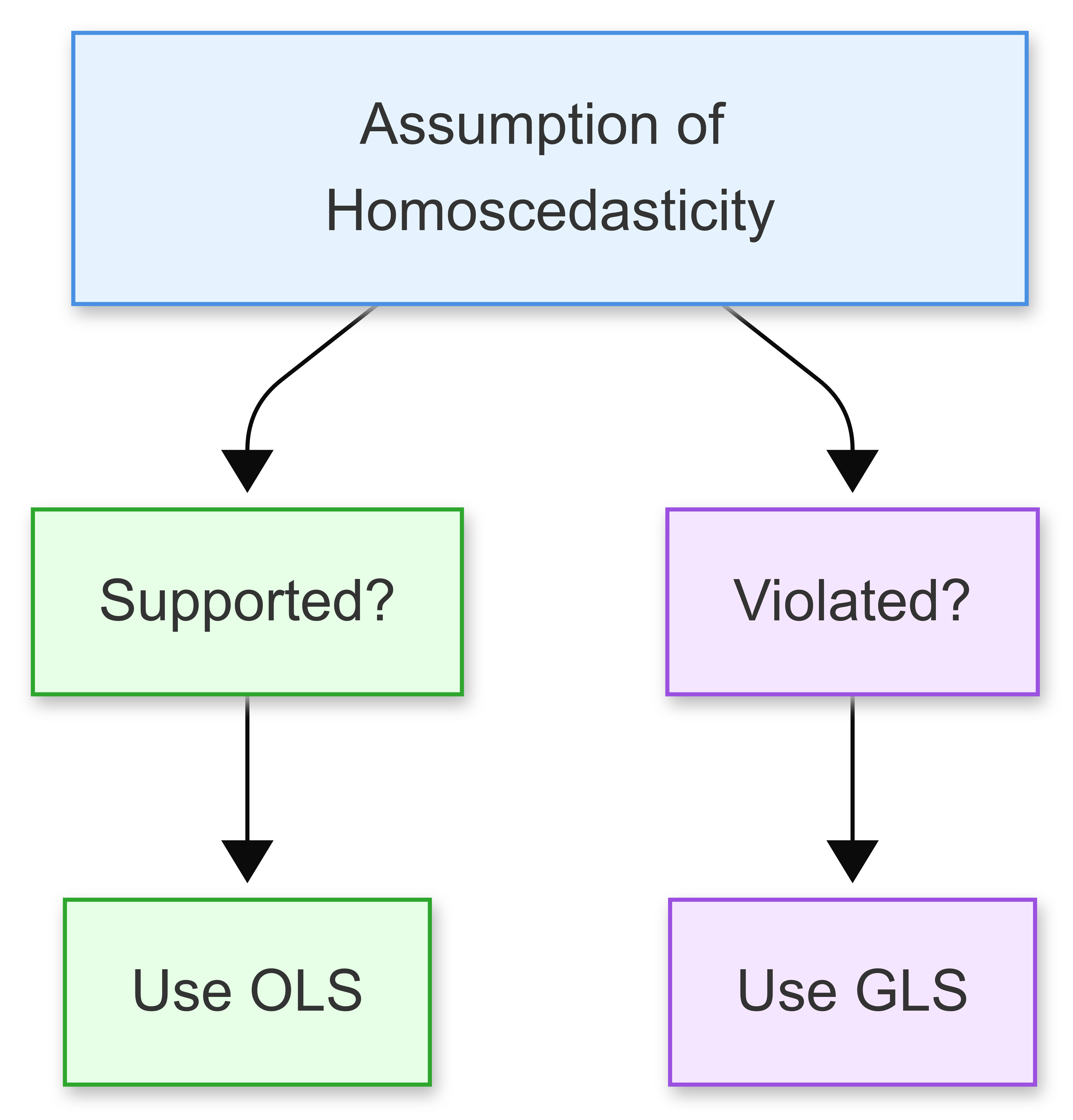
When the assumption of homoscedasticity is violated (i.e., the variance of the error terms is not constant, or when there is autocorrelation between the residuals) the Ordinary Least Squares estimates may no longer be efficient.
Generalised Least Squares (GLS) is an extension of OLS that allows for more flexibility in the error structure. It provides a way to handle heteroscedasticity and autocorrelation by transforming the model into one where the standard OLS techniques can be applied effectively.
Example
Suppose we are studying the previous income dataset, and we discover that the variance of income increases with age.
A GLS model can be formulated by first estimating the variance structure of the errors (perhaps variance increasing with age) and then transforming the model using this structure to stabilise the variance.
This transformation might involve weighting each observation by the inverse of its variance, leading to a new model where the transformed variables satisfy the OLS assumptions.
Further Reading
For a comprehensive treatment of GLS models, see:
Greene, W.H. (2018). Econometric Analysis, 8th Edition, Pearson. Chapter 9: Generalized Least Squares and Related Topics.
Wooldridge, J.M. (2020). Introductory Econometrics: A Modern Approach, 7th Edition, Cengage Learning. Chapter 8.4: Generalized Least Squares (GLS) Estimation.
6.3.3 Weighted Least Squares (WLS)
Weighted Least Squares (WLS) is a special case of GLS, and is used specifically to handle heteroscedastic errors.
In WLS, each term in the least squares equation is weighted by an inverse function of the variance of the observations, which helps in stabilising the variance across the data points.
This method is particularly useful when the error variance is a function of observable variables.
For example, if you’re measuring the impact of advertising spending on sales, the error variance might increase with the level of advertising spending. This means that predictions become less reliable (have more variance) at higher spending levels. In such cases, WLS can help by giving less weight to observations with higher variance.
Example
In the income prediction model, if we observe that the variance of income seems to be proportional to the square of age, we can use WLS by assigning weights to each observation. These weights could be the inverse of the predicted variance (e.g., \(1/Age^2\)).
The regression equation would then minimise the weighted sum of squared residuals, giving higher importance to observations where age is lower (assuming younger individuals have less income variability).
6.4 Model Diagnostics
6.4.1 Introduction
In multiple regression, the term ‘model diagnostics’ refers to a set of statistical techniques and methods we can use to evaluate the quality and validity of a regression model we have developed.
These diagnostics help us assess whether the model’s assumptions are met, and identify potential problems that could affect the reliability of the results.
The main objectives of model diagnostics include:
- Verifying the assumptions of linear regression (linearity, independence, homoscedasticity, normality) in our data;
- Identifying influential observations and outliers that might distort the results;
- Detecting potential model specification problems; and
- Assessing the model’s predictive accuracy and ‘goodness of fit’.
6.4.2 Residual analysis
Residual analysis is a tool for assessing the fit and appropriateness of the model assumptions.
Residuals, the differences between observed values and values predicted by the model, should ideally exhibit randomness and no pattern when plotted against predicted values or any independent variables.
Such patterns might indicate non-linearity, heteroscedasticity, or other model inadequacies. Plotting residuals can help identify outliers and influential points that may skew the regression analysis.
Key plots we might use include the residual plot, the standardised residual plot, and the normal probability plot. We would also want to check for autocorrelation in residuals, particularly in time series data, where this can be a significant issue.
.png)
.png)
6.4.3 Measures of influence
While all data points contribute to the formation of a regression model, some have a disproportionately large impact on the outcome.
Influence measures are crucial for identifying these points. Techniques such as leverage (hat) values, Cook’s distance, and DFBETAS are commonly used to assess the influence of individual data points on the estimated regression coefficients and the overall fit.
Identifying and scrutinising influential points help ensure that our model’s conclusions are not unduly driven by anomalies in the data.
6.4.4 Specification error tests
Specification error tests are vital for verifying the form and variables included in the regression model.
These tests check for the omission of relevant variables, the inclusion of irrelevant variables, and incorrect functional forms, common pitfalls in model specification that can lead to biased or inconsistent estimates.
Techniques such as the Ramsey RESET test help detect whether additional explanatory variables should be included in the model.
Tests like the link test or Wald test can determine if the model has been mis-specified due to incorrect functional forms or non-linear relationships that have not been accounted for.
Addressing specification errors is critical for ensuring the model’s appropriateness and the validity of its predictive power.
6.5 Model Selection
6.5.1 Introduction
Model selection is the process of choosing the most appropriate set of predictor variables from all available variables to create the best possible regression model.
This involves balancing model complexity with predictive accuracy to avoid both underfitting and overfitting.
Underfitting occurs when a model is too simple and fails to capture important patterns in the data. Overfitting happens when a model becomes too complex and starts to capture noise in the training data.
Example
For example, imagine we’re trying to predict a basketball player’s scoring average. We might have access to quite a few variables:
Minutes played per game;
Previous season’s scoring average;
Field goal attempts per game;
Height and weight;
Years of experience; and
Team’s pace of play.
While we could include all these variables in our model, some might not contribute meaningfully to predicting scoring average. Model selection helps us determine which combination of these variables creates the most effective predictive model while avoiding unnecessary complexity.
Various statistical criteria and techniques help us make this selection, including R-squared, adjusted R-squared, AIC, and BIC, which we explore in detail in the following sections.
6.5.2 R-squared and Adjusted R-squared
Introduction
R-squared and adjusted R-squared are commonly-used metrics for evaluating and comparing multiple regression models.
While both provide insights into how well a model explains the variability of the dependent variable, they have distinct applications and limitations in model selection.
R-Squared (\(R^2\))
\(R^2\) represents the proportion of variance in the dependent variable (y) that is explained by the independent variables (X1,X2,…,Xk) in our model.
It’s calculated as:
\[ R^2 = 1 - \frac{\text{SS}_{\text{residuals}}}{\text{SS}_{\text{total}}} \]
Where:
- \(SSresiduals\): Sum of squared residuals.
- \(SStotal\): Total sum of squares.
A higher \(R^2\) suggests that the model explains a greater proportion of variance. However, \(R^2\) always increases or remains the same when additional predictors are added to the model, even if the new predictors are irrelevant. This can lead to overfitting.
Adjusted R-Squared
\(R^2_{\text{adj}}\) adjusts \(R^2\) for the number of predictors in the model and the sample size.
It is given by:
\[ R^2_{\text{adj}} = 1 - \left( \frac{(1 - R^2)(n - 1)}{n - k - 1} \right) \]
Where:
- \(n\): Sample size.
- \(k\): Number of predictors.
\(R^2_{\text{adj}}\) penalises the addition of predictors that do not improve the model sufficiently. It only increases if the new predictor improves the model’s explanatory power more than would be expected by chance.
A higher \(R^2_{\text{adj}}\) indicates a better balance between explanatory power and model complexity.
Used in Model Selection
Evaluating Model Fit We use R^2 to assess the overall explanatory power of the model. For instance:
- If Model A has \(R^2=0.80\) and Model B has \(R^2=0.85\), Model B explains more variance in y.
Choosing Between Models
Use \(R^2_{\text{adj}}\) to decide whether adding predictors improves the model. For example:
- Model A: \(R^2\)=0.85, \(R^2_{\text{adj}}\)=0.82
- Model B: \(R^2\)=0.87, \(R^2_{\text{adj}}\)=0.83
Although R2 suggests Model B is better, the smaller increase in \(R^2_{\text{adj}}\) highlights that the additional predictor in Model B provides only a marginal benefit.
Parsimony
In practical applications, prioritising a higher \(R^2_{\text{adj}}\) often leads to simpler models that avoid overfitting. For example, adding a fourth predictor to a model might slightly increase \(R^2\) but decrease \(R^2_{\text{adj}}\), signaling that the predictor may not be worth including.
Example: Model Selection in Housing Price Prediction
Imagine you’re building a model to predict house prices (y) using the following predictors:
- X1: Square footage.
- X2: Number of bedrooms.
- X3: Distance to the nearest school.
- X4: Presence of a swimming pool.
| Model | \(R^2\) | \(R^2_{\text{adj}}\) |
|---|---|---|
| Model 1 (Square footage only) | 0.70 | 0.69 |
| Model 2 (+ Number of bedrooms) | 0.76 | 0.74 |
| Model 3 (+ Distance to school) | 0.78 | 0.75 |
| Model 4 (+ Swimming pool) | 0.79 | 0.74 |
Model 4 has the highest \(R^2\), but its \(R^2_{\text{adj}}\) decreases compared to Model 3, suggesting that the presence of a swimming pool does not improve the model significantly relative to its complexity.
In this case, Model 3 strikes the best balance between explanatory power and parsimony.
Limitations
- Nonlinear Relationships: \(R^2\) and \(R^2_{\text{adj}}\) are less meaningful for models with complex nonlinear relationships. Other metrics like Akaike Information Criterion (AIC) or Bayesian Information Criterion (BIC) may be more appropriate.
- Model Assumptions: Both metrics assume that the model satisfies key regression assumptions (e.g., linearity, homoscedasticity, no multicollinearity).
6.5.3 Akaike Information Criterion (AIC)
The Akaike Information Criterion (AIC) is widely used metric for model selection in statistical and ML. It was created by Hirotogu Akaike.
It gives us a way to compare different models based on how well they fit the data while penalising model complexity.
The AIC is calculated as:
\[ AIC=2k−2ln(L) \]
where \(k\) represents the number of model parameters, and \(L\) is the likelihood of the model given the data.
Lower AIC values indicate a better balance between goodness of fit and model simplicity.
AIC and Model Comparison
When comparing multiple models, the one with the lowest AIC is generally preferred, as it suggests the best trade-off between explanatory power and overfitting. However, AIC doesn’t directly test the quality of a model, but rather ranks competing models relative to each other.
Unlike hypothesis testing methods (e.g., likelihood ratio test) AIC does not provide a probability or significance level; instead, it helps identify the model that minimises information loss.
6.5.4 Bayesian Information Criterion (BIC)
The Bayesian Information Criterion (BIC) is another metric used for model selection, similar to the Akaike Information Criterion (AIC), but with a stronger penalty for complexity.
It’s calculated as:
\[ BIC=kln(n)−2ln(L) \]
where \(k\) is the number of model parameters, \(n\) is the sample size, and \(L\) is the likelihood of the model. The logarithmic dependence on \(n\) makes BIC penalise additional parameters more heavily than AIC, favouring simpler models when sample sizes are large.
BIC and Model Comparison
Like AIC, BIC is used to compare models, with the model having the lowest BIC being preferred. The key difference is that BIC’s stronger penalty on complexity makes it more likely to select a simpler model, particularly in large datasets.
Remember: With AIC and BIC, lower is generally a better model.
This aligns with Bayesian principles, as BIC incorporates the idea of model likelihood while accounting for the probability of overfitting. However, BIC does not provide a formal hypothesis test; it’s a ranking method for selecting the most parsimonious model.
Using BIC
BIC is widely used in regression analysis, time series modelling, and machine learning, especially when selecting among nested models. It’s particularly useful when dealing with large datasets where the risk of overfitting is high.
While AIC is more flexible and often used in exploratory modelling, BIC tends to be more conservative and favours models that generalise well to new data. In practice, both AIC and BIC are often computed together to assess the trade-offs between model complexity and predictive performance.
6.6 Testing Assumptions
6.6.1 Introduction
As we have discussed, testing assumptions helps ensure the validity and reliability of our statistical model. When we perform multiple regression, we make several key assumptions about our data and the relationships between variables.
These assumptions include the normality of residuals, homoscedasticity (constant variance), and independence of errors. If these assumptions are violated, our regression results may be biased or unreliable, leading to incorrect conclusions.
Understanding and testing these assumptions allows us to:
- Validate the accuracy of our regression models
- Identify potential problems in our data or analysis
- Make necessary adjustments or transformations when assumptions are violated
- Draw more reliable conclusions from our statistical analyses
In the following sections, we’ll explore each of these assumptions in detail and learn how to test them effectively.
6.6.2 Normality of residuals
As we have covered, in regression analysis a key assumption is that the residuals (the differences between observed and predicted values) follow a normal distribution.
This assumption is particularly important for statistical inference, as it ensures that confidence intervals and hypothesis tests are valid. When residuals are normally distributed, regression coefficients and their associated p-values can be interpreted correctly.
Deviations from normality may indicate that the model is missing important variables, nonlinear relationships, or heteroscedasticity (unequal variance).
6.6.3 Checking Normality of Residuals
There are several methods to check the normality of residuals. Visual methods include histograms, Q-Q plots (quantile-quantile plots), and density plots:
.png)
Statistical tests such as the Shapiro-Wilk test and the Kolmogorov-Smirnov test can provide formal assessments:
.png)
Note that statistical tests can be sensitive to sample size. Small datasets may fail to detect non-normality, while large datasets may flag minor deviations that are not practically significant. Therefore, a combination of visual inspection and statistical testing is generally recommended.
6.6.4 Homoscedasticity
Homoscedasticity, also known as homogeneity of variance, is a fundamental assumption in many statistical analyses, particularly in regression and ANOVA.
It refers to the condition where the variability of a dependent variable is equal across the range of values of an independent variable that predicts it.
In simpler terms, when we plot our data, the spread of the residuals (the differences between observed and predicted values) should be fairly consistent across all levels of our predictor variables. This assumption is crucial because when it’s violated (heteroscedasticity), it can lead to unreliable statistical inferences and incorrect standard errors.
When heteroscedasticity is present, it often manifests as a pattern in your residual plots, such as a fan or cone shape. This can occur for various reasons, including the presence of outliers, skewed distributions, or an inherent relationship between the variance and the mean of your data.undefined
.png)
To address heteroscedasticity, we might employ several solutions including data transformation (such as logarithmic transformation), weighted least squares regression, or robust standard errors.
6.6.5 Independence of errors
The independence of errors assumption in regression analysis states that residuals (errors) should not be correlated with one another.
This means that the value of one residual should not provide information about the value of another. Violating this assumption, particularly in time-series data or spatial data, can lead to misleading statistical inferences, such as underestimated standard errors and inflated significance levels. When errors are correlated (autocorrelated), the model may not capture all underlying patterns in the data, indicating a need for adjustments.
6.6.6 Detecting violations of independence
One of the ways to check for independence of errors is through a residual plot, where residuals should appear randomly scattered without any visible pattern.
.png)
Additionally, in time-series analysis, autocorrelation can be assessed using the Durbin-Watson test, where a value close to 2 suggests little to no autocorrelation, while values closer to 0 or 4 indicate positive or negative correlation, respectively. We’ll cover this later in the module.
.png)